Graph Neural Networks (GNNs)
GCN and GAT Python Implementation
In the world of artificial intelligence, where data is the lifeblood that fuels innovation, there’s a particular type of data that often challenges traditional machine learning techniques, data with inherent relationships and connections. This is where Graph Neural Networks (GNNs) step in, revolutionizing the way we process and understand data structured as graphs.
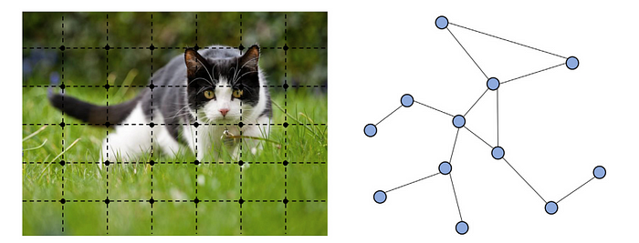
As a unique non-Euclidean data structure for machine learning, graph analysis focuses on tasks such as node classification, link prediction, and clustering. In a world that can be visualized as networks of entities and their interactions, be it social networks, molecular structures, recommendation systems, or citation networks, traditional machine learning algorithms often fall short. Conventional models are designed for independent and identically distributed data, struggling to capture the nuances of interconnectedness and dependencies that define these complex relationships.

Graph Neural Networks have emerged as a revolutionary approach, garnering significant attention in recent years due to their remarkable capacity to extract invaluable insights from interconnected data. Unlike traditional methods that focus solely on individual data points in isolation, GNNs operate by delving deep into the intricate tapestry of relationships. This unique approach empowers us to not only analyze data points but to unravel the concealed structures and intricate patterns that lay beneath the surface.
In this blog, our focus will be on dissecting the fundamental operational architecture of Graph Neural Networks (GNNs), coupled with a practical exploration of their implementation using the Python programming language. Through this journey, we aim to demystify the inner workings of GNNs, providing you with a clear understanding of how these networks navigate and make sense of interconnected data. So, let’s embark on a guided tour of the core concepts behind GNNs, while also rolling up our sleeves for some hands-on Python coding to bring these concepts to life.
Getting Started
Let’s examine the Planetoid Cora dataset and apply Graph Neural Networks (GNNs) using PyTorch. This practical exploration will provide us with hands-on experience working with real-world graph data.
The Planetoid dataset combines citation networks from Cora, CiteSeer, and PubMed. Nodes, representing documents, feature 1433-dimensional bag-of-words vectors, interconnected by citations. With 7 classes, the challenge involves training a model to predict missing labels using the web of connections.
from torch_geometric.datasets import Planetoid
from torch_geometric.transforms import NormalizeFeatures

dataset = Planetoid(root='data/Planetoid', name='Cora', transform=NormalizeFeatures())

print(f'Dataset: {dataset}:')
print('======================')
print(f'Number of graphs: {len(dataset)}')
print(f'Number of features: {dataset.num_features}')
print(f'Number of classes: {dataset.num_classes}')

data = dataset[0]
print(data)
Output =
Dataset: Cora():
======================
Number of graphs: 1
Number of features: 1433
Number of classes: 7
Data(x=[2708, 1433], edge_index=[2, 10556], y=[2708], train_mask=[2708], val_mask=[2708], test_mask=[2708])Prior to initiating the training process, let’s analyze the data distribution by visually representing it within the second and third dimensions.
Just one more step to go. Now, it’s time to write the classes and methods that will be employed in the upcoming sections:
class BuildModel():
    def __init__(self, model, lr = 0.01):
        self.model = model
        self.optimizer = torch.optim.Adam(model.parameters(), lr=lr, weight_decay=5e-4)
        self.criterion = torch.nn.CrossEntropyLoss()

    def single_train(self):
          self.model.train()
          self.optimizer.zero_grad()
          out = self.model(data.x, data.edge_index)
          loss = self.criterion(out[data.train_mask], data.y[data.train_mask])
          loss.backward()
          self.optimizer.step()
          return loss

    def test(self):
          self.model.eval()
          out = self.model(data.x, data.edge_index)
          pred = out.argmax(dim=1)
          test_correct = pred[data.test_mask] == data.y[data.test_mask]
          test_acc = int(test_correct.sum()) / int(data.test_mask.sum())
          return test_acc

    def train_with_early_stopping(self, epochs=150, patience=10, plot = False, plot_name = None):

        history = {
            'epoch': [],
            'loss': [],
            'test_acc': []
        }

        best_test_acc = 0.0
        epochs_without_improvement = 0

        for epoch in range(1, epochs + 1):
            loss = self.single_train()
            test_acc = self.test()

            print(f'Epoch: {epoch:03d}, Loss: {loss:.4f}, Test Acc: {test_acc:.4f}')

            history['epoch'].append(epoch)
            history['loss'].append(loss.item())
            history['test_acc'].append(test_acc)

            if test_acc > best_test_acc:
                best_test_acc = test_acc
                epochs_without_improvement = 0
            else:
                epochs_without_improvement += 1

            if epochs_without_improvement >= patience:
                print(f'Early stopping triggered at epoch {epoch}.')
                break

        if plot:
            self.history_plot(history, plot_name)

        return history

    def train(self, epoch = 100):
        for epoch in range(1, epochs + 1):
            loss = self.single_train()
            test_acc = self.test()

            print(f'Epoch: {epoch:03d}, Loss: {loss:.4f}, Test Acc: {test_acc:.4f}')


    def history_plot(self, history, plot_name):
        fig = go.Figure()
        fig.add_trace(go.Scatter(x=history['epoch'], y=history['loss'], mode='lines', name='Training Loss'))
        fig.add_trace(go.Scatter(x=history['epoch'], y=history['test_acc'], mode='lines', name='Test Accuracy'))
        fig.update_layout(
            title='Training History',
            xaxis_title='Epoch',
            yaxis_title='Value',
            legend=dict(x=0, y=1),
            template='plotly_dark'
        )
        fig.show()
Following that, we proceed to define our visualization methods:
def visualize_2d(h, color, name = '2D_dist_plot'):
    z = TSNE(n_components=2).fit_transform(h.detach().cpu().numpy())

    fig = px.scatter(x=z[:, 0], y=z[:, 1], color=color, color_continuous_scale="magma")
    fig.update_layout(
        xaxis_title="Dimension 1",
        yaxis_title="Dimension 2",
        xaxis=dict(showgrid=False, zeroline=False, showticklabels=False),
        yaxis=dict(showgrid=False, zeroline=False, showticklabels=False),
        coloraxis_showscale=False,
        width=800,
        height=800
    )
    fig.show()


def visualize_3d(h, color, name = '3D_dist_plot'):
    z = TSNE(n_components=3).fit_transform(h.detach().cpu().numpy())

    fig = px.scatter_3d(x=z[:, 0], y=z[:, 1], z=z[:, 2], color=color, color_continuous_scale="magma")
    fig.update_layout(
        scene=dict(
            xaxis_title="Dimension 1",
            yaxis_title="Dimension 2",
            zaxis_title="Dimension 3"
        ),
        coloraxis_showscale=False,
        width=800,
        height=800
    )
    fig.show()
Now let’s delve into the exciting world of Graph Neural Networks (GNNs) and explore how we can use them to train our dataset.
1. Graph Convolutional Network (GCN)
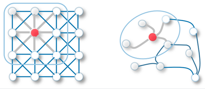
A Graph Convolutional Network (GCN) is a Graph Neural Network (GNN) variant tailored for processing graph-structured data. Unlike Convolutional Neural Networks (CNNs), which excel at grid-like data (such as images), GCNs specialize in datasets where entities are connected through edges, forming networks.
While CNNs leverage local patterns in grid data, GCNs harness the interconnectedness of graph data. They propagate and aggregate information across neighboring nodes, updating each node’s representation based on its neighbors’ features. This contextual understanding enables GCNs to capture relationships and patterns.

The notable shift in GCNs lies in adapting the convolutional operation for graphs. This operation computes weighted averages of neighboring node features, generating central node representations. As these layers stack, GCNs learn abstract features while considering the overall graph context.
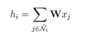
In the realm of traditional neural networks, linear layers play a pivotal role by applying a fundamental linear transformation to the input data. This transformation holds the power to metamorphose the input features denoted as x into a fresh realm of hidden vectors, which are symbolized as h. This enchanting metamorphosis is orchestrated through the agency of a weight matrix 𝐖, an omnipresent protagonist in this neural narrative. Disregarding the role of biases for this moment of elucidation, we can elegantly express this process as follows:

One way to enhance our node representations is by combining their features with those of their neighboring nodes. This process, known as convolution or neighborhood aggregation, involves incorporating information from the immediate neighborhood of a node, including the node itself (denoted as Ñ).

Unlike CNN filters, in Graph Neural Networks (GNNs), our weight matrix 𝐖 is singular and shared across all nodes. However, a challenge arises due to the variable number of neighbors nodes can have, unlike the fixed grid structure of pixels in CNNs. This distinction is a key aspect of GNNs that enables them to effectively operate on graph-structured data.
How should we handle situations in which a single node is connected to only one neighbor, while another node has 700 connections? If we were to merely combine the feature vectors, the resultant embedding ‘h’ would be disproportionately influenced by the 700-neighbor node. To ensure uniform value ranges across all nodes and enable meaningful comparisons between them, we can normalize the output according to the nodes’ degrees (the count of connections each node possesses).

The researchers noted that attributes originating from nodes with a high degree of neighbors spread more effortlessly compared to those from relatively secluded nodes. In order to counterbalance this phenomenon, they proposed the idea of assigning greater weights to attributes from nodes with limited neighbors. This strategy aims to harmonize the impact across the entire node network. This process can be expressed as follows:

Let’s implement the concepts we’re discussing in Python using PyTorch for a deeper understanding.
First, let’s build the GCN model using PyTorch:
from torch_geometric.nn import GCNConv

class GCN(torch.nn.Module):
    def __init__(self, hidden_channels):
        super().__init__()
        torch.manual_seed(1234567)
        self.conv1 = GCNConv(dataset.num_features, hidden_channels)
        self.conv2 = GCNConv(hidden_channels, dataset.num_classes)

    def forward(self, x, edge_index):
        x = self.conv1(x, edge_index)
        x = x.relu()
        x = F.dropout(x, p=0.5, training=self.training)
        x = self.conv2(x, edge_index)
        return x

model = GCN(hidden_channels=16)
print(model)
>>>GCN(
>>> (conv1): GCNConv(1433, 16)
>>> (conv2): GCNConv(16, 7)
>>>)Once we have built our model, we can move on to training and visualizing it:
model = GCN(hidden_channels=16)

built_model = BuildModel(model)
Epoch: 001, Loss: 1.9463, Test Acc: 0.2700
Epoch: 002, Loss: 1.9409, Test Acc: 0.2910
Epoch: 003, Loss: 1.9343, Test Acc: 0.2910
Epoch: 004, Loss: 1.9275, Test Acc: 0.3210
Epoch: 005, Loss: 1.9181, Test Acc: 0.3630
Epoch: 006, Loss: 1.9086, Test Acc: 0.4120
Epoch: 007, Loss: 1.9015, Test Acc: 0.4010
Epoch: 008, Loss: 1.8933, Test Acc: 0.4020
Epoch: 009, Loss: 1.8808, Test Acc: 0.4180
Epoch: 010, Loss: 1.8685, Test Acc: 0.4470
Epoch: 011, Loss: 1.8598, Test Acc: 0.4680
Epoch: 012, Loss: 1.8482, Test Acc: 0.5180
Epoch: 013, Loss: 1.8290, Test Acc: 0.5440
Epoch: 014, Loss: 1.8233, Test Acc: 0.5720
Epoch: 015, Loss: 1.8057, Test Acc: 0.5910
Epoch: 016, Loss: 1.7966, Test Acc: 0.6080
Epoch: 017, Loss: 1.7825, Test Acc: 0.6300
Epoch: 018, Loss: 1.7617, Test Acc: 0.6450
Epoch: 019, Loss: 1.7491, Test Acc: 0.6520
Epoch: 020, Loss: 1.7310, Test Acc: 0.6560
Epoch: 021, Loss: 1.7147, Test Acc: 0.6570
Epoch: 022, Loss: 1.7056, Test Acc: 0.6640
Epoch: 023, Loss: 1.6954, Test Acc: 0.6770
Epoch: 024, Loss: 1.6697, Test Acc: 0.6950
Epoch: 025, Loss: 1.6538, Test Acc: 0.7140
Epoch: 026, Loss: 1.6312, Test Acc: 0.7150
Epoch: 027, Loss: 1.6161, Test Acc: 0.7170
Epoch: 028, Loss: 1.5899, Test Acc: 0.7230
Epoch: 029, Loss: 1.5711, Test Acc: 0.7220
Epoch: 030, Loss: 1.5576, Test Acc: 0.7210
Epoch: 031, Loss: 1.5393, Test Acc: 0.7280
Epoch: 032, Loss: 1.5137, Test Acc: 0.7370
Epoch: 033, Loss: 1.4948, Test Acc: 0.7380
Epoch: 034, Loss: 1.4913, Test Acc: 0.7430
Epoch: 035, Loss: 1.4698, Test Acc: 0.7510
Epoch: 036, Loss: 1.3998, Test Acc: 0.7570
Epoch: 037, Loss: 1.4041, Test Acc: 0.7600
Epoch: 038, Loss: 1.3761, Test Acc: 0.7640
Epoch: 039, Loss: 1.3631, Test Acc: 0.7700
Epoch: 040, Loss: 1.3258, Test Acc: 0.7800
Epoch: 041, Loss: 1.3030, Test Acc: 0.7810
Epoch: 042, Loss: 1.3119, Test Acc: 0.7760
Epoch: 043, Loss: 1.2519, Test Acc: 0.7760
Epoch: 044, Loss: 1.2530, Test Acc: 0.7790
Epoch: 045, Loss: 1.2492, Test Acc: 0.7800
Epoch: 046, Loss: 1.2205, Test Acc: 0.7790
Epoch: 047, Loss: 1.2037, Test Acc: 0.7850
Epoch: 048, Loss: 1.1571, Test Acc: 0.7900
Epoch: 049, Loss: 1.1700, Test Acc: 0.7920
Epoch: 050, Loss: 1.1296, Test Acc: 0.7940
Epoch: 051, Loss: 1.0860, Test Acc: 0.7930
Epoch: 052, Loss: 1.1080, Test Acc: 0.7910
Epoch: 053, Loss: 1.0564, Test Acc: 0.7930
Epoch: 054, Loss: 1.0157, Test Acc: 0.7930
Epoch: 055, Loss: 1.0362, Test Acc: 0.7920
Epoch: 056, Loss: 1.0328, Test Acc: 0.7980
Epoch: 057, Loss: 1.0058, Test Acc: 0.8000
Epoch: 058, Loss: 0.9865, Test Acc: 0.7970
Epoch: 059, Loss: 0.9667, Test Acc: 0.8010
Epoch: 060, Loss: 0.9741, Test Acc: 0.8000
Epoch: 061, Loss: 0.9769, Test Acc: 0.8030
Epoch: 062, Loss: 0.9122, Test Acc: 0.8040
Epoch: 063, Loss: 0.8993, Test Acc: 0.8050
Epoch: 064, Loss: 0.8769, Test Acc: 0.8050
Epoch: 065, Loss: 0.8575, Test Acc: 0.8060
Epoch: 066, Loss: 0.8897, Test Acc: 0.8030
Epoch: 067, Loss: 0.8312, Test Acc: 0.8060
Epoch: 068, Loss: 0.8262, Test Acc: 0.8030
Epoch: 069, Loss: 0.8511, Test Acc: 0.8070
Epoch: 070, Loss: 0.7711, Test Acc: 0.8070
Epoch: 071, Loss: 0.8012, Test Acc: 0.8080
Epoch: 072, Loss: 0.7529, Test Acc: 0.8080
Epoch: 073, Loss: 0.7525, Test Acc: 0.8070
Epoch: 074, Loss: 0.7689, Test Acc: 0.8110
Epoch: 075, Loss: 0.7553, Test Acc: 0.8140
Epoch: 076, Loss: 0.7032, Test Acc: 0.8120
Epoch: 077, Loss: 0.7326, Test Acc: 0.8110
Epoch: 078, Loss: 0.7122, Test Acc: 0.8120
Epoch: 079, Loss: 0.7090, Test Acc: 0.8110
Epoch: 080, Loss: 0.6755, Test Acc: 0.8130
Epoch: 081, Loss: 0.6666, Test Acc: 0.8070
Epoch: 082, Loss: 0.6679, Test Acc: 0.8080
Epoch: 083, Loss: 0.7037, Test Acc: 0.8100
Epoch: 084, Loss: 0.6752, Test Acc: 0.8070
Epoch: 085, Loss: 0.6266, Test Acc: 0.8100
Early stopping triggered at epoch 85.
2. Graph Attention Networks (GAT)
GAT stands for Graph Attention Network, and it’s a type of Graph Neural Network (GNN) that has gained significant attention due to its effectiveness in modeling relationships within graph-structured data. GAT was introduced by Velickovic et al. in their 2018 paper “Graph Attention Networks.”
GAT addresses one of the key challenges in GNNs, which is how to effectively aggregate information from neighboring nodes in a graph while assigning different levels of importance to different neighbors. Traditional GNNs, such as Graph Convolutional Networks (GCNs), use fixed aggregation schemes that treat all neighbors equally. GAT, on the other hand, introduces the concept of attention mechanisms into the aggregation process, allowing each node to dynamically weigh the importance of its neighbors’ information.
GAT Layer
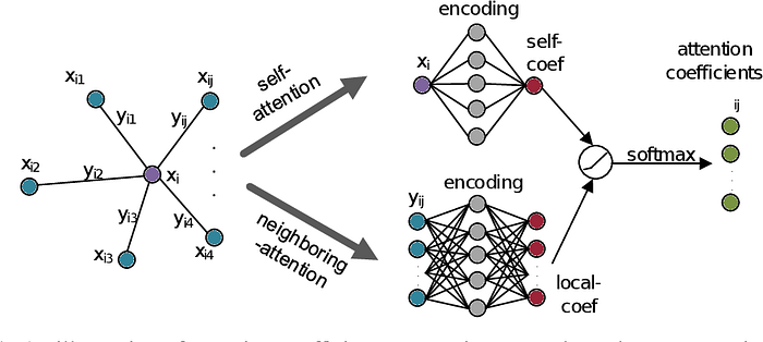
In this step, a shared, linear transformation takes center stage, embodied by the matrix W with dimensions (F’, F). This transformation is aptly named “shared” because every individual node undergoes the same W matrix-based transformation.
The mission here is to harmonize the dimensionality of node features. Originally of dimension F, these features are transformed to a uniform dimensionality of F’. This transformation is systematically applied to all nodes in node i’s neighborhood, encompassing node i itself.

During this process, the embedding representation h_i of the target node i is fused with the embeddings of its immediate neighbors. Each pairing is then combined and transformed using matrix W^a, which is characterized by its dimensions (2F’, F’) here, F’ might stay the same or differ from the previous stage based on a hyperparameter.
The central aim here is to facilitate a collective learning of attention between these pairs of nodes, bypassing the specifics of the graph structure.

Here, each intermediate attention scalar comes to life through a non-linear activation, denoted as σ. In the GAT research, the authors opt for LeakyReLU as their chosen non-linear activation function.
Wrapping things up, the energized intermediate attention scalars flow through a softmax layer. This transformation imbues the attention coefficients with the properties of a probability distribution.
In essence, this phase centers on the normalization of attention coefficients, aligning them for further processing.


The attention mechanism utilized by our model is defined by a parametric weight vector. This weight vector is associated with a LeakyReLU activation function, contributing to the overall functionality of the mechanism.
Consider an illustrative example of multihead attention with the scenario where K equals 3 heads. In this case, we focus on node 1 within its local neighborhood. Distinct styles and colors of arrows symbolize separate computations of attention, each operating independently. The outcomes from each head’s attention calculation are then combined by means of concatenation or averaging. This fusion of features results in the final representation denoted as h1'.

Put differently, employing this approach allows us to observe the operational dynamics of the Graph Attention Network (GAT).

Let’s put these concepts we discussed into practice using PyTorch in Python to develop a deeper understanding.
from torch_geometric.nn import GATConv

class GAT(torch.nn.Module):
    def __init__(self, hidden_channels, heads):
        super().__init__()
        torch.manual_seed(1234567)
        self.conv1 = GATConv(dataset.num_features, hidden_channels,heads)
        self.conv2 = GATConv(heads*hidden_channels, dataset.num_classes,heads)

    def forward(self, x, edge_index):
        x = F.dropout(x, p=0.6, training=self.training)
        x = self.conv1(x, edge_index)
        x = F.elu(x)
        x = F.dropout(x, p=0.6, training=self.training)
        x = self.conv2(x, edge_index)
        return x

model = GAT(hidden_channels=8, heads=8)
print(model)
GAT(
(conv1): GATConv(1433, 8, heads=8)
(conv2): GATConv(64, 7, heads=8)
)Now, we should proceed with training and also visualize our GAT model:
buildGANModel = BuildModel(model, lr = 0.05)
history = buildGANModel.train_with_early_stopping(plot = True, plot_name = 'gat_history_plot')
Epoch: 001, Loss: 0.6564, Test Acc: 0.7780
Epoch: 002, Loss: 0.6479, Test Acc: 0.7780
Epoch: 003, Loss: 0.6208, Test Acc: 0.8100
Epoch: 004, Loss: 0.5841, Test Acc: 0.8180
Epoch: 005, Loss: 0.5878, Test Acc: 0.8170
Epoch: 006, Loss: 0.5477, Test Acc: 0.8060
Epoch: 007, Loss: 0.4723, Test Acc: 0.7950
Epoch: 008, Loss: 0.4452, Test Acc: 0.8000
Epoch: 009, Loss: 0.4338, Test Acc: 0.8070
Epoch: 010, Loss: 0.4332, Test Acc: 0.8100
Epoch: 011, Loss: 0.4218, Test Acc: 0.8150
Epoch: 012, Loss: 0.3900, Test Acc: 0.8150
Epoch: 013, Loss: 0.4190, Test Acc: 0.8160
Epoch: 014, Loss: 0.4238, Test Acc: 0.8080
Early stopping triggered at epoch 14.Feel free to click here to access the entire code.
That concludes my blog. I trust that you found it impactful. I’m open to both positive and negative feedback, so please don’t hesitate to share your thoughts. Your feedback is eagerly anticipated. Stay committed and dedicated.
References
- https://www.datacamp.com/tutorial/comprehensive-introduction-graph-neural-networks-gnns-tutorial
- https://www.youtube.com/watch?v=SnRfBfXwLuY
- https://nabila-abraham.medium.com/ohmygraphs-graph-attention-networks-b7562289ae4b
- https://towardsdatascience.com/graph-convolutional-networks-introduction-to-gnns-24b3f60d6c95
- Petar Veličković (2018). Graph Attention Networks. https://arxiv.org/pdf/1710.10903.pdf
- Jie Zhou (2020). Graph neural networks: A review of methods and applications. https://arxiv.org/ftp/arxiv/papers/1812/1812.08434.pdf
